Strangeworks Workflows

🧩

Beta Release

Workflows is currently in beta and access is limited to selected participants. If you do not yet have access but are interested in trying Workflows, please apply for the beta here. Not all users will have access at this time.

What is Workflows?

Strangeworks Workflows is a user-friendly platform that enables you to build, solve, and analyze complex mathematical optimization problems—no programming required.

• No- & Low-Code Modeling
  Express your optimization objectives and constraints in plain language. There is no need to write mathematical formulas or code.

• AI-Powered Model Translation
  Workflows interprets your descriptions and translates them into precise mathematical models, such as Mixed Integer Programming (MIP) and Quadratic Unconstrained Binary Optimization (QUBO).

• Seamless Model Execution
  Run your models on a wide range of classical and quantum computing resources using the Strangeworks compute catalog.

• Integrated AI Assistance
  Get guidance and support at every stage, from model creation to solution analysis.

Workflows is built for optimization professionals, quantitative analysts, and decision-makers with mathematical backgrounds, as well as organizations seeking to address complex challenges in areas like resource allocation, planning, and scheduling. Whether you are working independently or as part of a team, Workflows offers a flexible environment to model, experiment, and solve advanced optimization scenarios efficiently.

Key Features

• AI-powered model development agent and chatbot
  Accelerate model creation and refinement with natural language interaction, making advanced optimization accessible to both experts and teams.

• Integrated lab book environment for computational science projects
  Organize your work in a structured workspace that brings together problem formulation, data, constraints, and solver configuration—ideal for collaborative research and enterprise experimentation.

• Backend-agnostic execution via the Strangeworks compute catalog
  Seamlessly access both classical and quantum solvers, empowering users to experiment with a wide range of optimization engines and approaches.

These features are crafted to support the workflows of professionals and organizations aiming to experiment, iterate, and deploy optimization solutions efficiently and effectively.

• For SDK-based optimization, see Strangeworks Optimization package.

Workflows is designed to guide you through the entire optimization process, from initial idea to actionable results. Here’s an overview of the typical steps you’ll follow:

1. Describe Your Problem
   Enter your optimization goal in natural language (e.g., "minimize delivery costs"). Workflows translates this into a mathematical model.

2. Generate & Refine Model
   The system builds an initial model from your prompt and data (e.g., MIP, QUBO). Edit or iterate as needed.

3. Add Data
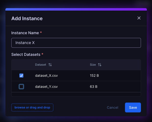
   Import or create datasets (distance matrices, cost tables, etc.) to define your scenario.

4. Configure Instances
   Pair your model with datasets to create specific problem instances.

   Note: Once an instance is created, its model is locked. Duplicate the model to refine further without affecting existing results.

5. Select Solver & Parameters
   Choose a solver (e.g., Simulated Annealing, Gurobi, Toshiba) and adjust parameters if needed.

   Tip: Defaults work for most cases. For tuning, see parameter guides.

6. Run Optimization
   Start the solver. The platform manages the job and results appear when ready.

7. Review & Iterate
   Analyze results and visualizations. Refine your model or data and repeat as needed.

This end-to-end workflow allows you to move seamlessly from problem definition to solution, supporting experimentation and rapid iteration—all within a single, integrated environment.

Getting Started

Setup

Workspace Access

• Ensure you have access to an active Strangeworks workspace with the Workflows feature enabled.
• If you're new to Strangeworks, learn how the platform works first.

Credits

• Problem instance submission and execution requires compute credits, which are deducted when running models on solvers.
• Workflows execution consumes compute credits based on the selected solver and problem complexity. Monitor your credit balance and review solver pricing before execution. Learn more about billing and credits.

Project Setup

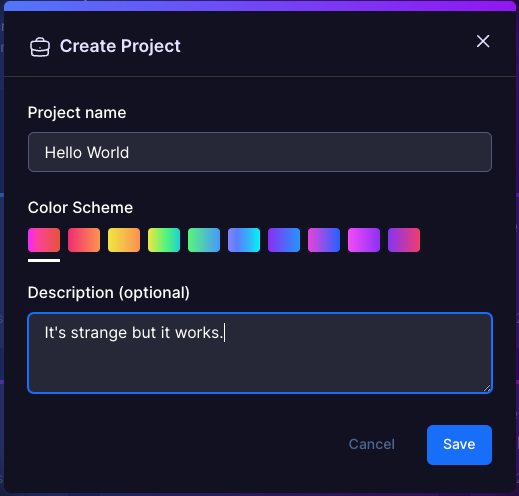
• Create a new project inside the workspace or join one started by a team mate and collaborate.
• Projects help organize your optimization work and can contain multiple problems, models, datasets, and solver runs.

info

Simulators provide a low-cost way to test and validate your optimization model before committing compute credits to a production solver. Use a simulator to quickly check your model's logic, constraints, and data integration. Once you are satisfied with the results, you can confidently run your instance on a full solver for final results.

Problem Definition

The best way to understand Workflows is to dive right in with a classic optimization problem. Let's start with the Traveling Salesman Problem (TSP) – a foundational challenge in optimization that's both intuitive and powerful.

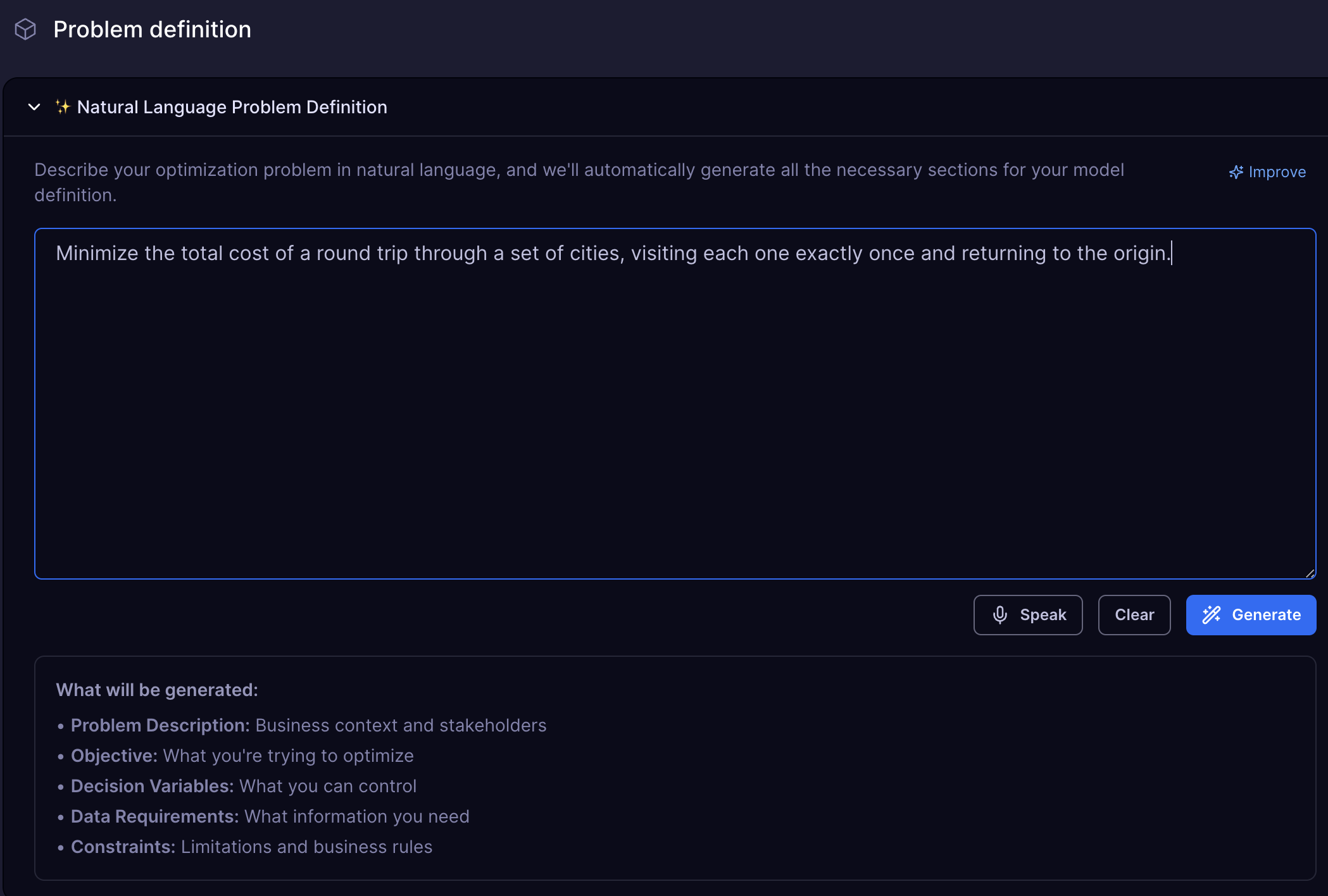
Your First Prompt: Think of a delivery driver who needs to visit multiple cities in the most efficient way possible. Here's how you'd describe this to Workflows:

PROMPT

Minimize the total cost of a round trip through a set of cities, visiting each one exactly once and returning to the origin.

This simple sentence contains everything Workflows needs to understand your optimization goal. Notice how it naturally captures:

• The objective: minimize total cost
• The constraint: visit each city exactly once
• The structure: round trip (returning to start)

✨ Improve

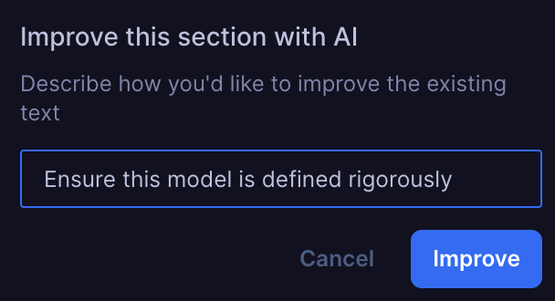
Refining your prompt before generating a model can help Workflows better understand your intent and increase the chances of obtaining a high-quality solution on the first attempt.

Once you click Generate, Workflows transforms your natural language into a mathematical model. The platform analyzes your description and generates the underlying optimization framework, complete with decision variables, constraints, and objective functions.

💡 Getting Started

1. Create a new project in Workflows.
2. Enter the TSP prompt:
   "Minimize the total cost of a round trip through a set of cities, visiting each one exactly once and returning to the origin."
3. Observe how Workflows automatically translates your description into a mathematical optimization model, complete with variables, constraints, and an objective function, ready to be solved.

Model Structure

Model Classification

🛠 Problem Types

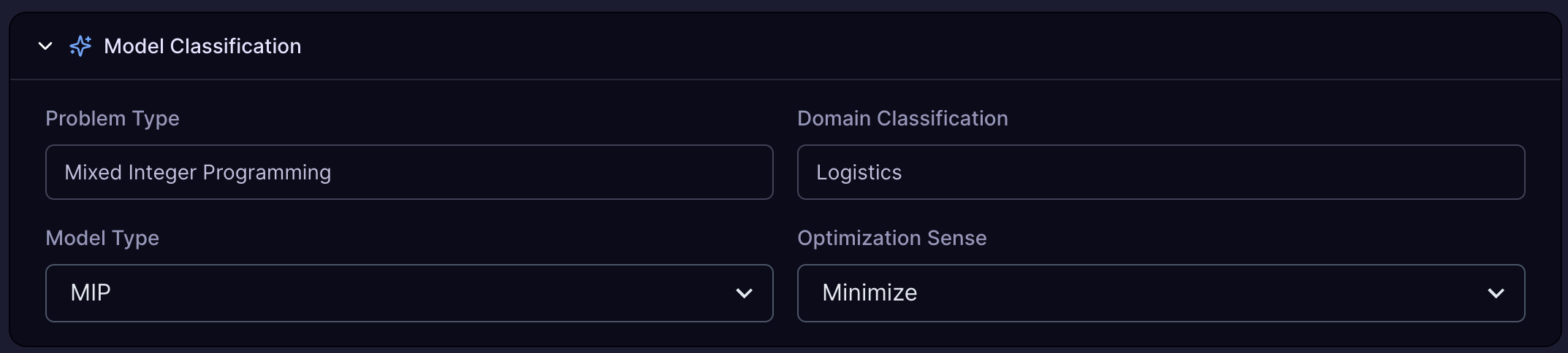
MIP (Mixed Integer Programming) is recommended for most optimization problems. QUBO (Quadratic Unconstrained Binary Optimization) is more experimental and offers access to quantum solvers, which may be more powerful for certain types of problems.

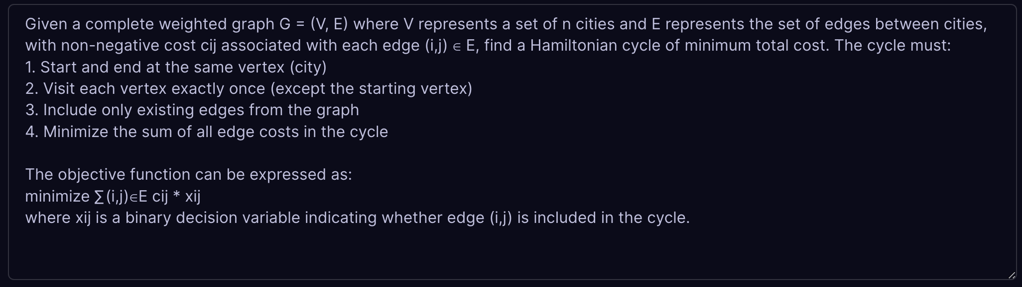
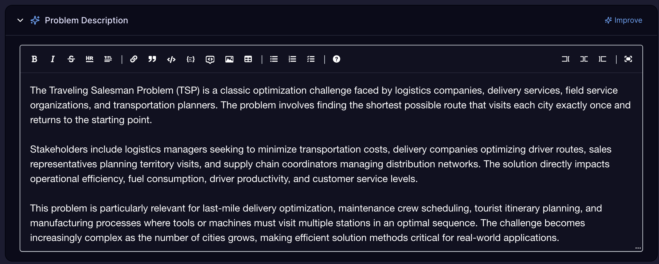
Problem Description

Problem description provides a high-level overview of the problem you are trying to solve. It is used to classify the problem and to generate a model.

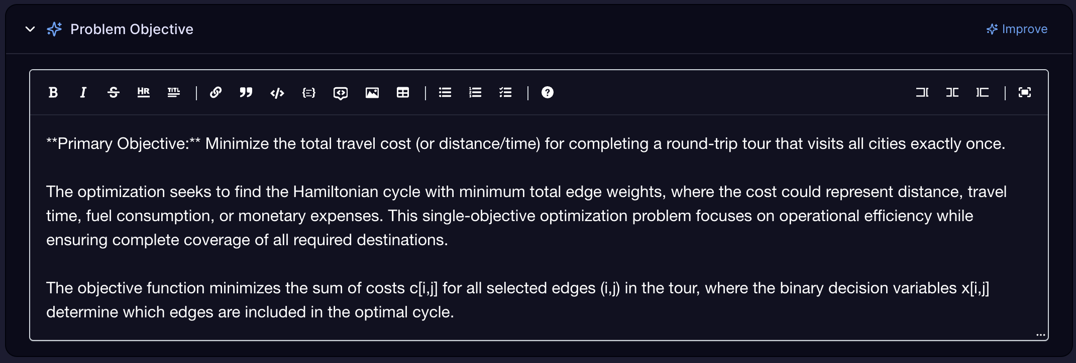
Problem Objective

The objective function is the number you are trying to minimize or maximize.

Problem Data

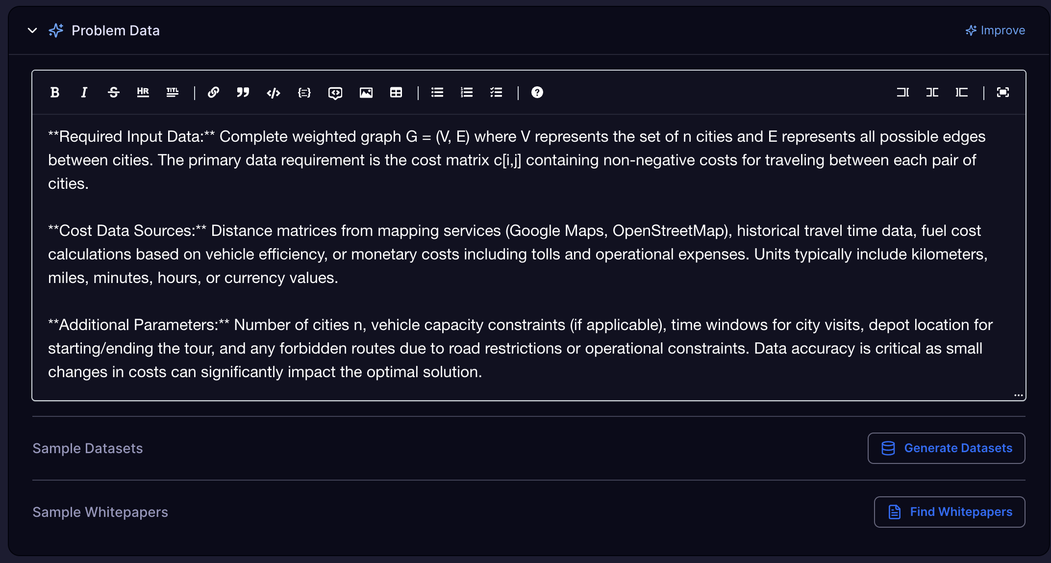
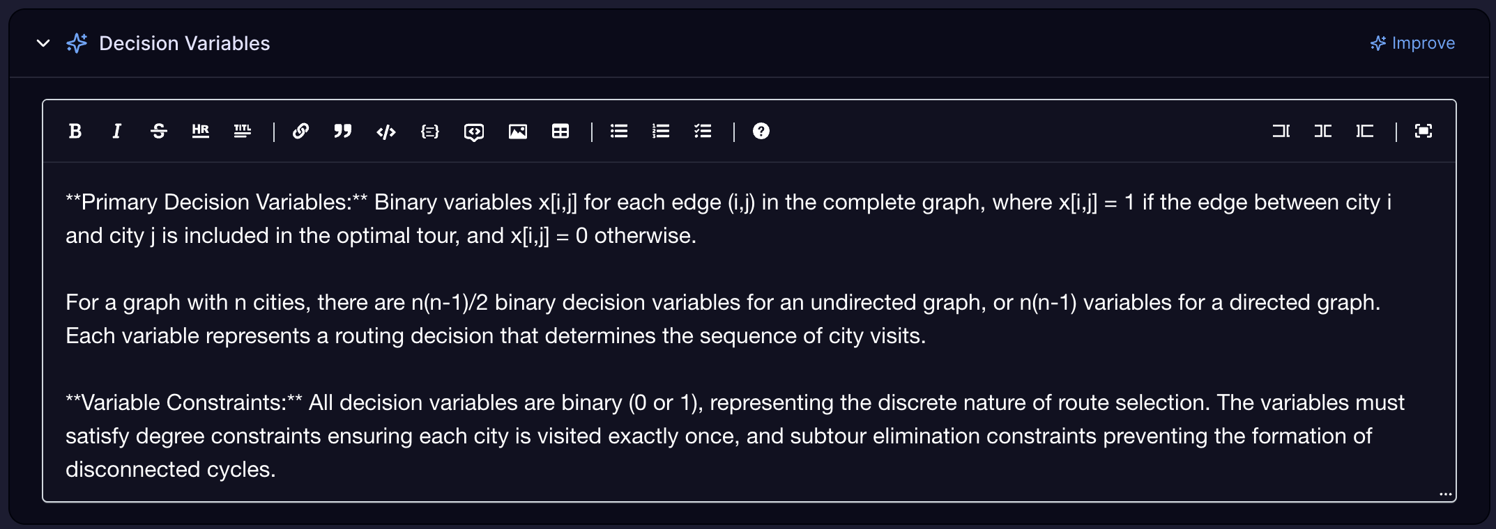
Decision Variables

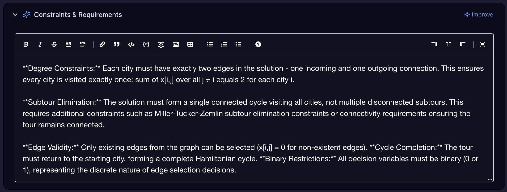
Constraints and Requirements

Generated Models

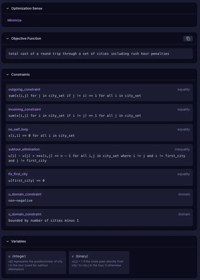
After parsing the Model Viewer shows:

• Objective functions - The goal you're trying to optimize (minimize cost, maximize profit, etc.)

• Decision variables - The values the solver can change to find the optimal solution

• Constraints - Rules and limitations that must be satisfied in the solution

• Cost and penalty components - Weights and penalties that guide the optimization

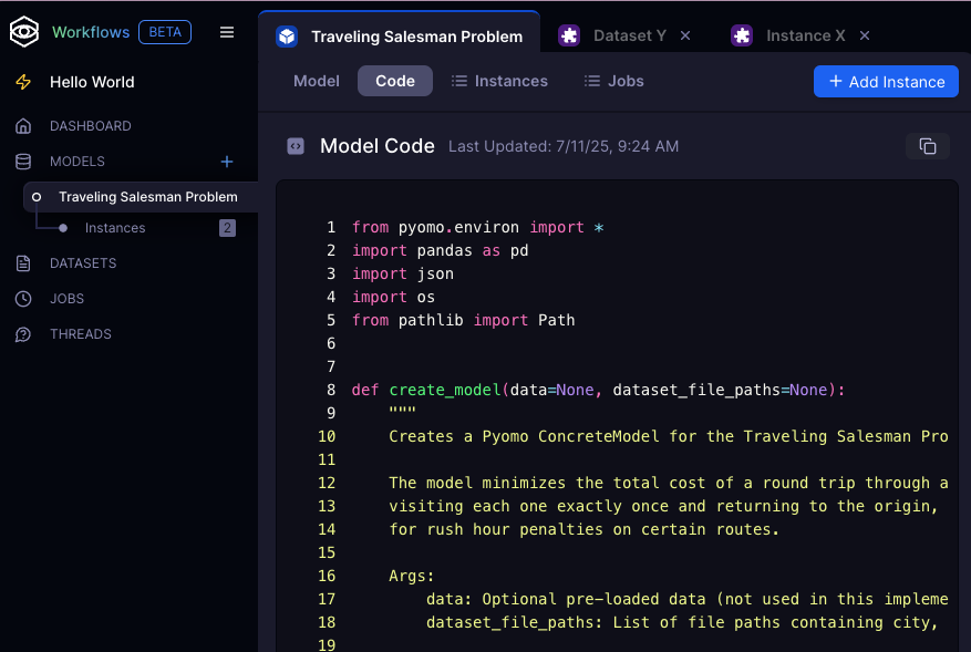
• A data-agnostic model template: This abstract representation defines the structure of your optimization problem—its variables, constraints, and objectives—without tying it to any specific dataset.

• A Python-based modeling object (using Pyomo): This is a programmatic version of your model, suitable for advanced users who wish to inspect or extend the underlying mathematical formulation.

  

Editing Models

You can modify your optimization model by updating:

• Problem Description
  • "Add a constraint that limits overtime to 10 hours per week."
  • "Change the objective to maximize total profit instead of minimizing cost."
  • "Set the variable representing the number of trucks to be an integer between 1 and 10."
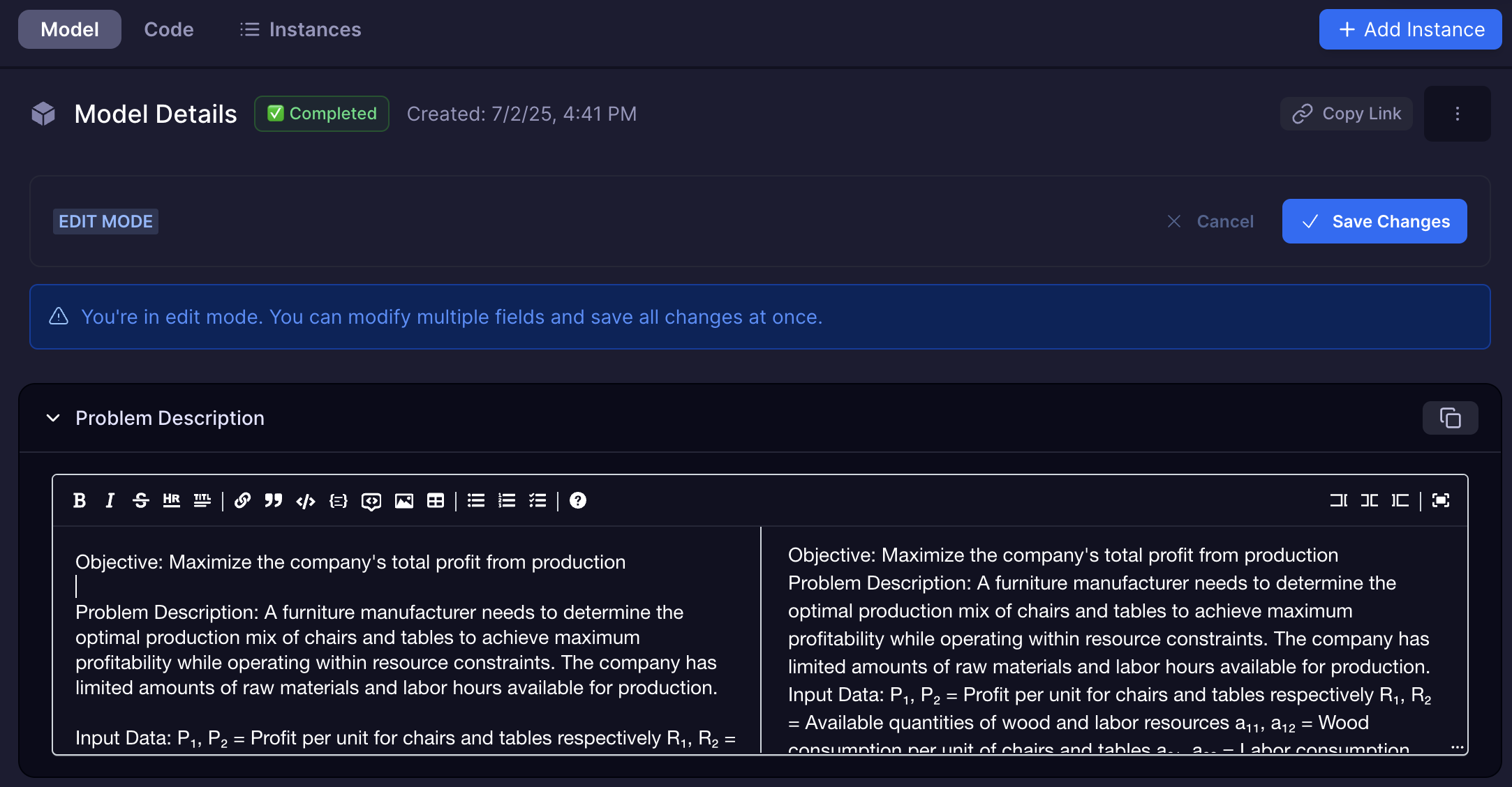
• Domain Classification
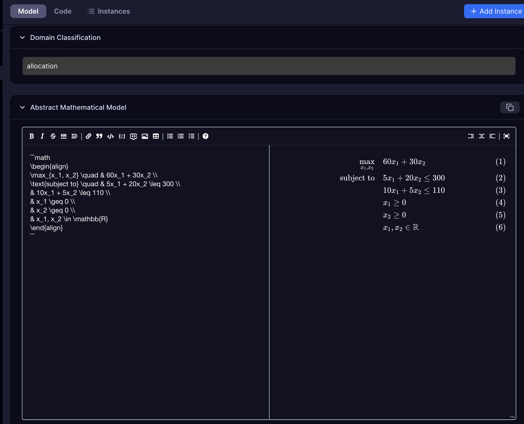
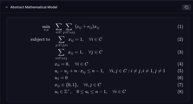
• Abstract Mathematical Model
• Optimization sense
• Objective Function
  • Adjust the objective function to align with your goals (e.g., minimize cost, maximize efficiency).
• Constraints
  • Add, remove, or refine constraints to better capture your requirements.
• Variables
  • Change variable types and bounds, such as specifying whether a variable should be continuous, integer, or binary.

Using Data

Now that we have the problem set up lets use a dataset (JSON, CSV) to create an instance.

Concept	Description
Model	Encodes the structure of the problem — constraints, variables, and objective logic
Dataset	Encodes the specifics — the distance matrix, city names, costs, etc
Instance	A pairing of the two — ready to solve

When solving a simple Traveling Salesperson Problem (TSP), you might ask:

"Why not just describe the whole problem — cities, distances, everything — in the prompt?"

And you'd be right, for small, static problems, this works fine. The model and the data are tightly coupled, and you effectively have a one-off instance.

In fact, this example demonstrates:

• constraint definitions
• cost function expression
• model-instance separation

By keeping the models and instances separate:

• You can reuse the same model across datasets
• You can benchmark new data without changing logic
• You can iterate on logic without rewriting data
• You can scale from toy problems to real-world scenarios

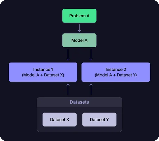
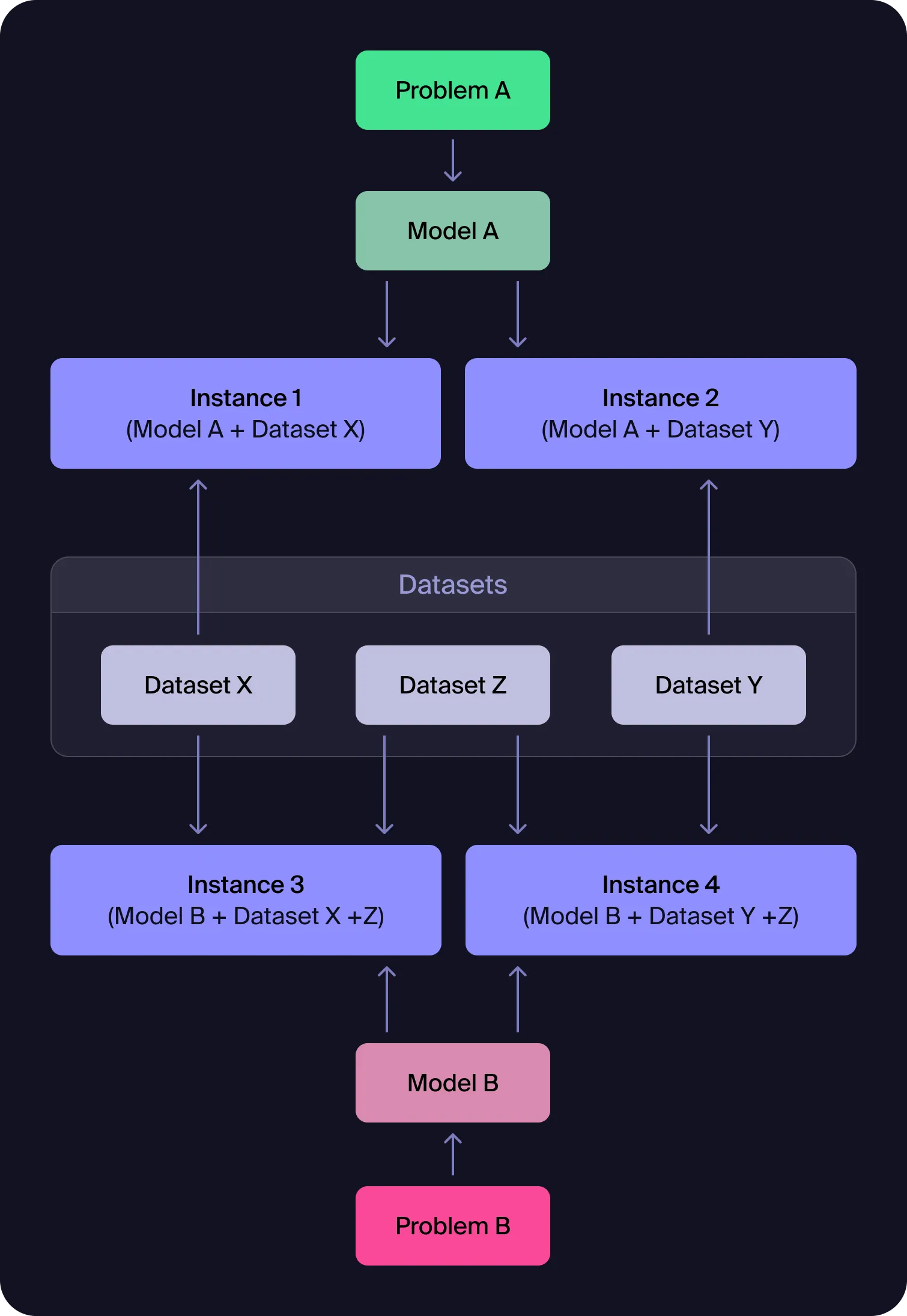
Figure 1: Model-Dataset-Instance Relationship
This diagram illustrates the fundamental architecture of Workflows: a single model (derived from your prompt) can be paired with multiple datasets to create different problem instances. Each instance represents a specific scenario that can be solved independently, enabling you to test the same optimization logic across various data configurations.

Dataset X: Symmetric and Dense

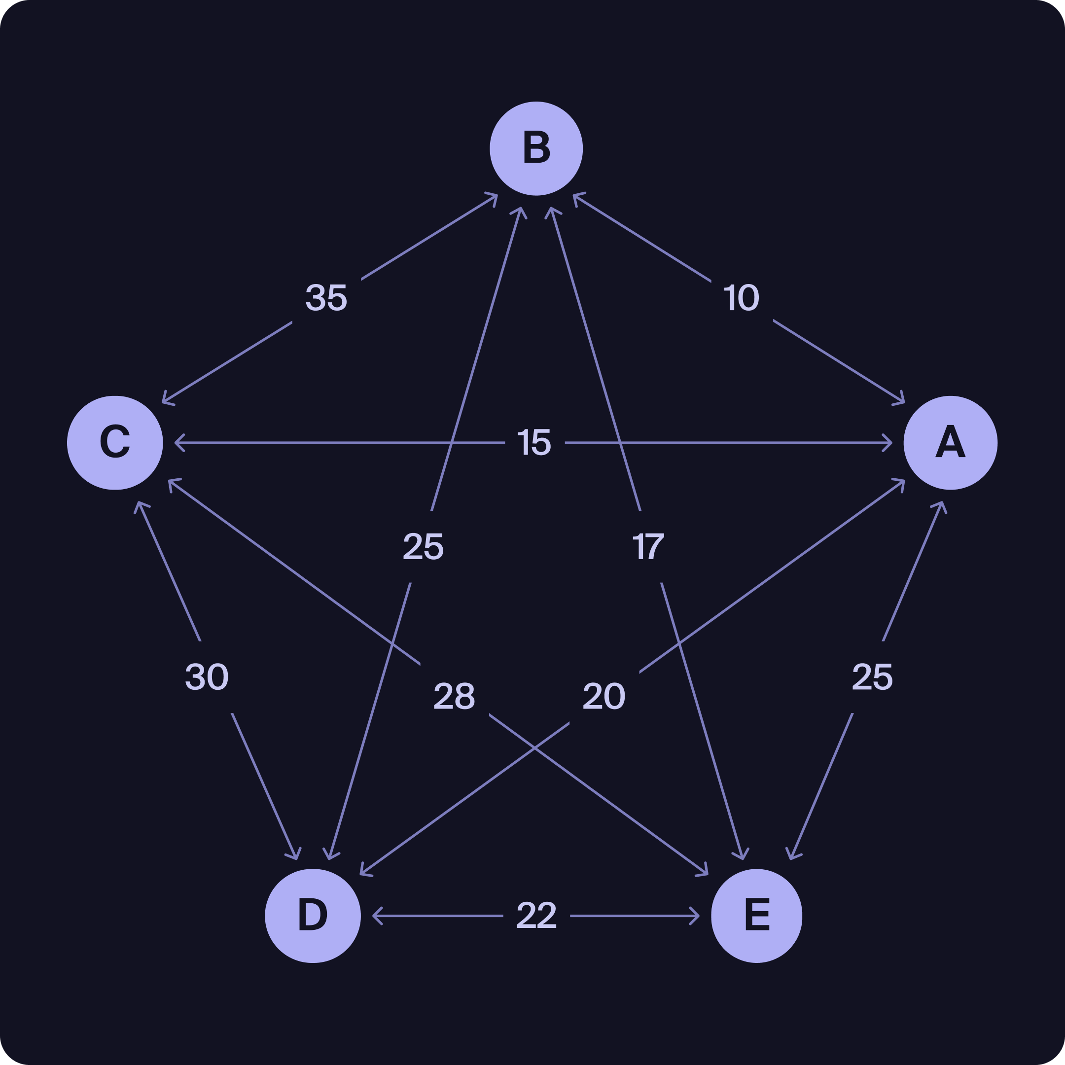
Dataset X Sample (Symmetric cost matrix):

from,to,cost
A,B,10
A,C,15
A,D,20
A,E,25
B,A,10
B,C,35
B,D,25
B,E,17
C,A,15
C,B,35
C,D,30
C,E,28
D,A,20
D,B,25
D,C,30
D,E,22
E,A,25
E,B,17
E,C,28
E,D,22

Dataset Y: Sparse and Asymmetric

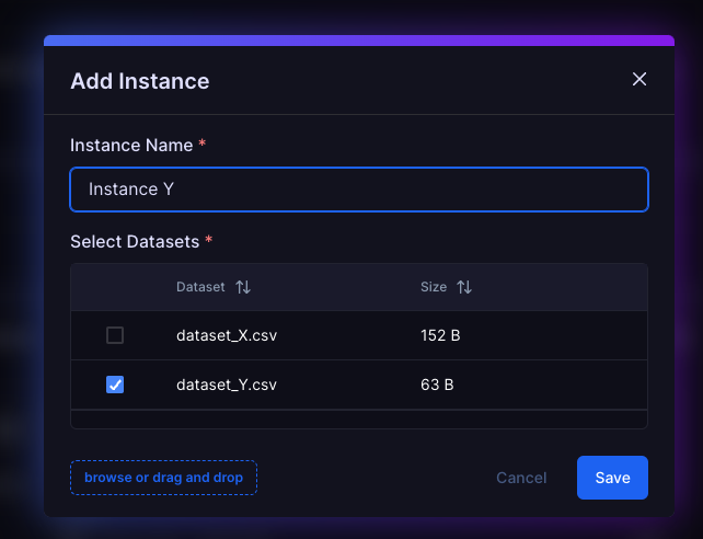
Dataset Y Sample (Sparse, asymmetric):

from,to,cost
A,B,7
B,C,9
C,D,11
D,E,6
E,A,14
A,C,18
B,D,8
C,E,5

Dataset Y represents an asymmetric graph—the cost from one node to another may differ from the reverse direction, and not all connections are present. This is important when modeling problems where travel costs or routes are not the same in both directions.

Feasibility

In some instances, the constraints you specify may be so strict that no feasible solution exists. When this happens, it may be necessary to relax certain constraints or prioritize them to find a workable solution.

Notice how in the graph for Dataset Y it is not possible to follow a non-repeating cycle that visits all nodes. This is because the graph is not Hamiltonian.

Solving Problems

Problem Instances

An instance is a specific scenario or case of your optimization problem, created by combining your model (the problem definition) with a particular dataset (the input data). Each instance represents a concrete problem to be solved by the optimization engine.

For example:

Instance 1: "Traveling Salesperson Problem" model + Dataset X (dense, symmetric distance matrix)

Instance 2: "Traveling Salesperson Problem" model + Dataset Y (sparse, asymmetric distance matrix)

You can create multiple instances to explore how your model performs with different datasets, constraints, or parameter settings. This flexibility allows you to compare results, test robustness, and iterate on your problem formulation—even in cases where your constraints are so strict that there may not even be a feasible solution.

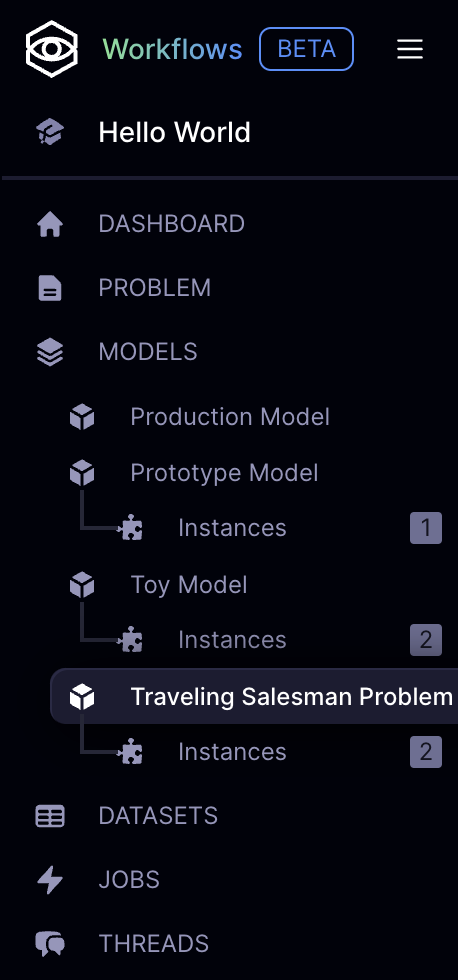
Project Dashboard

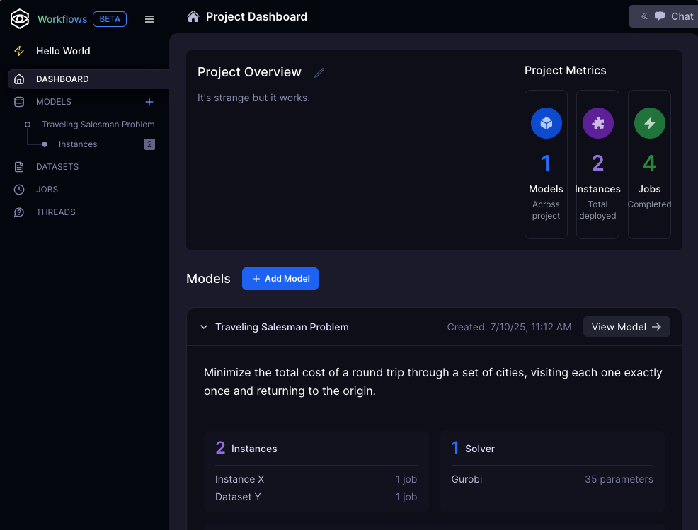
Manage:

• chat threads
• models
• instances
• datasets
• jobs

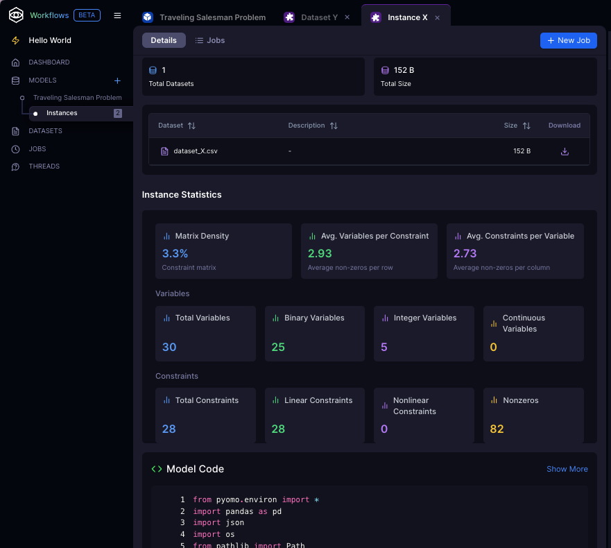
Instance Page

• Submit and review jobs
• Inspect instance statistics
• Refactor model code
• Download executable files

Solving Instances

After defining your model and creating one or more instances with specific datasets, you are ready to solve these instances using an optimization solver. The process is straightforward:

1. Select a Solver
   Choose the optimization engine (e.g., Quantagonia, Gurobi) that best fits your problem. Different solvers may offer unique strengths or support for specific problem types.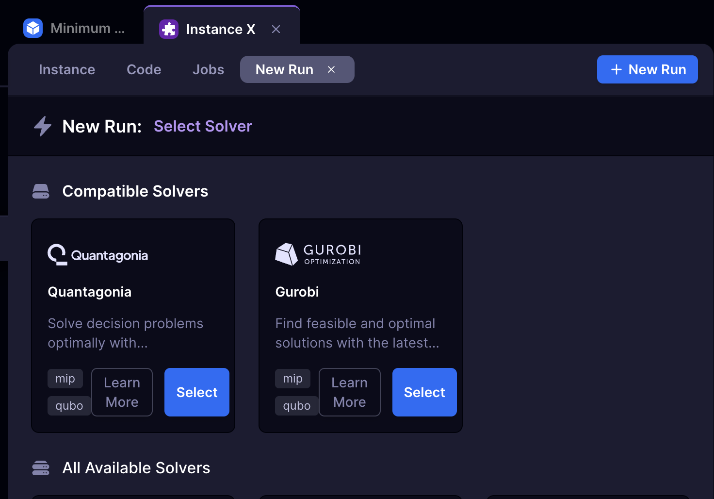

2. Configure Parameters
   Start with the default parameter settings, which are optimized for most cases. If needed, adjust options such as time limits, solution precision, or algorithmic strategies to suit your problem’s size and complexity.
   

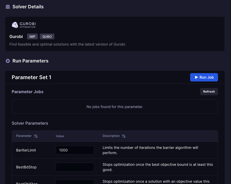
   • For more information on solver parameters, consult our providers documentation.

3. Run the Solver
   Launch the optimization. The system will monitor progress and provide updates in real time.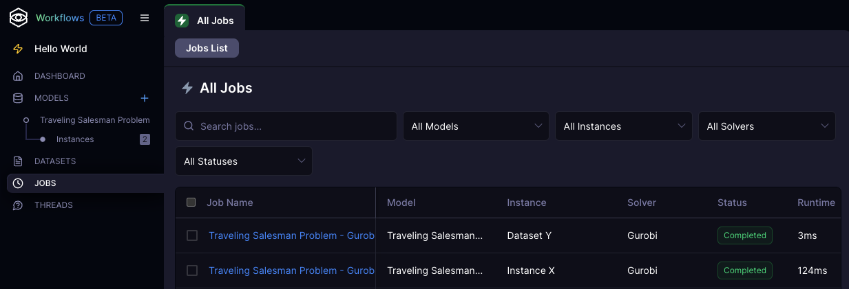

4. Review Results
   Once complete, examine the results pane for a summary of the solution, objective value, and additional insights. Use these results to refine your model or solver settings as needed.

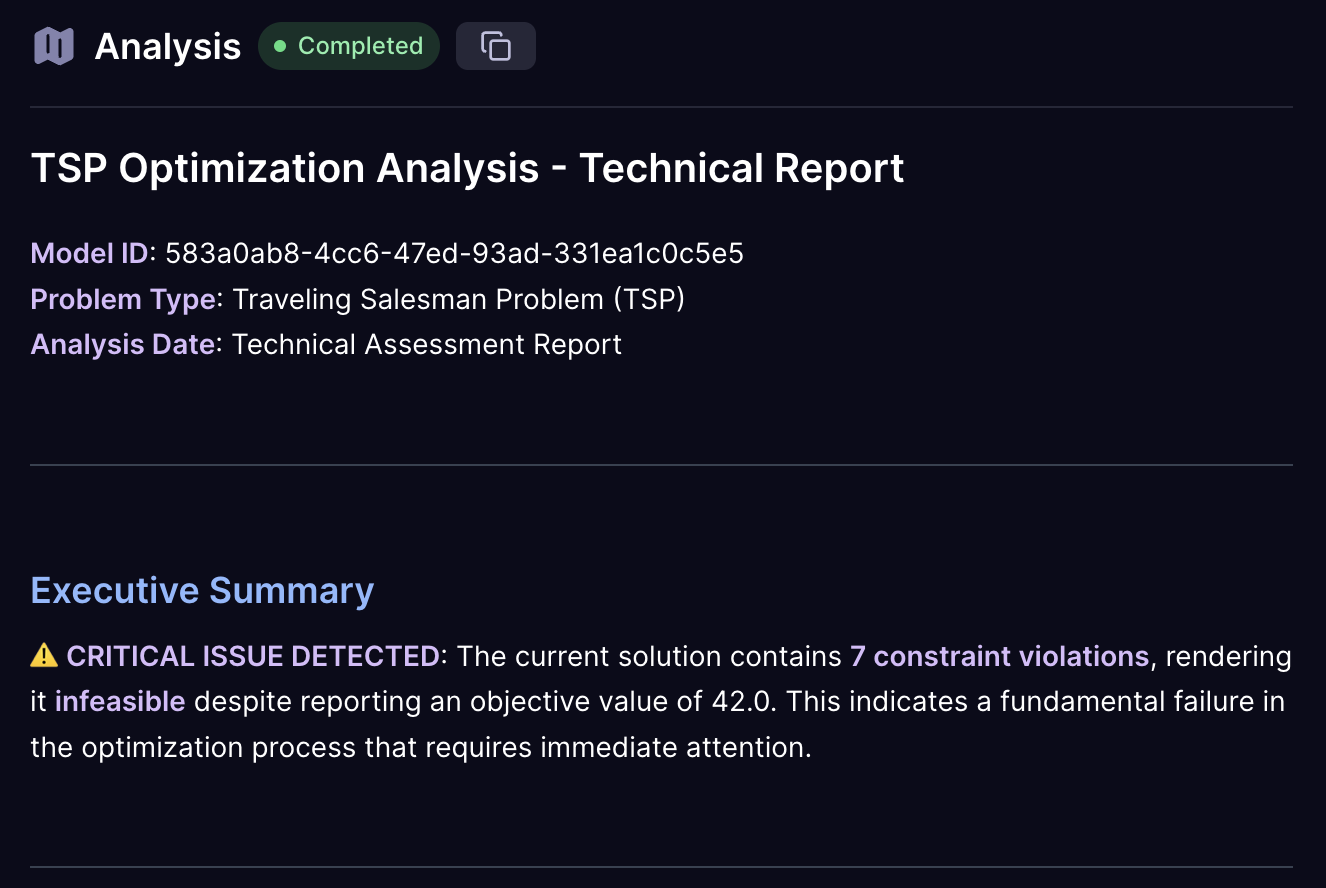
Results Analysis

Once your optimization completes, the Results pane provides comprehensive analysis tools to understand and interpret your solution. The results are organized into several key sections:

• Analysis
  • Executive Summary
  • Solution Quality Assessment
  • Constraint Violation Analysis
  • Solution Interpretation
  • Performance Analysis
  • Critical Issues Identified
  • Recommendations
  • Conclusion

• Results
  • Cost
  • Runtime
  • Objective Value

• Recommendations
• Constraints
  • Description
  • Violated Constraints
• Solver Parameters

Feasibility

Sometimes your optimization results will indicate that no feasible solution exists. This happened with Dataset Y from our earlier example, where the sparse, asymmetric graph structure doesn't allow for a valid Hamiltonian cycle. When the results analysis shows "infeasible" or identifies critical constraint violations, this presents an opportunity to refine your model.

Consider the case where Dataset Y produces an infeasible result for our strict TSP formulation. The results interpretation might show:

• Critical Issues Identified: No valid route exists that visits each city exactly once
• Constraint Violation Analysis: Hamiltonian cycle constraint cannot be satisfied
• Recommendations: Relax constraints or modify problem formulation

This feedback guides you toward a model refinement that handles the constraint more gracefully:

Original Constraint:

"Minimize the total cost of a round trip through a set of cities, visiting each one exactly once and returning to the origin."

Refined Constraint for Non-Hamiltonian Graphs:

"Minimize the total cost of a route through a set of cities, visiting each one at least once and returning to the origin. If a complete cycle isn't possible, find the minimum cost path that covers all cities with the fewest revisits."

This refinement transforms the problem from a strict Hamiltonian cycle requirement to a more flexible routing problem that can handle incomplete graphs. The model can now:

• Adapt to data constraints: Work with both complete and incomplete connection matrices
• Provide feasible solutions: Even when strict constraints cannot be satisfied
• Maintain optimization focus: Still minimize cost while ensuring all locations are visited

By using the results interpretation as a guide, you learn to identify when constraints are too restrictive for your data and develop more robust problem formulations that can handle real-world scenarios.

Adding Datasets

One of Workflows' most powerful features is the ability to evolve your optimization problems from simple academic examples to rich, realistic models that capture the nuances of real-world decision-making. This iterative approach allows you to start with a basic problem structure and progressively add layers of complexity, constraints, and contextual data without losing the core problem logic.

The separation of model logic from data is fundamental to this approach. Your initial model establishes the mathematical framework—the decision variables, objective function, and core constraints. As you iterate, you can enhance this foundation by introducing additional datasets that represent real-world complications, seasonal variations, or operational constraints that weren't obvious in your initial formulation.

Consider the evolution from textbook problems to production-ready models. A basic Traveling Salesman Problem might start with simple distance-based costs between cities. While this captures the essential structure, real-world routing involves time-dependent factors, vehicle capacity constraints, delivery windows, road restrictions, and dynamic costs that vary throughout the day.

From Simple to Sophisticated: The Rush Hour Example

Let's trace how a simple optimization problem becomes more realistic through iterative refinement:

Phase 1: Foundation Model

Your initial prompt establishes the core problem:

"Minimize the total cost of a round trip through a set of cities, visiting each one exactly once and returning to the origin."

This creates a clean mathematical framework focused on the essential optimization challenge. The model understands decision variables (which routes to take), the objective (minimize total cost), and the fundamental constraints (visit each city exactly once).

Phase 2: Adding Real-World Complexity

Once your foundation works, you can introduce the complexities that make the problem more realistic:

"Minimize the total cost of a round trip through a set of cities, visiting each one exactly once and returning to the origin. Some roads are busier during rush hour and incur an additional penalty if used. Account for this contextual data in the cost function with an additional input for rush penalties."

This enhancement transforms the problem from a static optimization to one that reflects dynamic real-world conditions. The rush hour penalties represent the reality that identical routes can have vastly different costs depending on timing, traffic patterns, and operational constraints.

The Power of Layered Datasets The elegance of this approach lies in how different datasets contribute distinct aspects of the problem:

• Base Datasets (X/Y) provide the fundamental structure: distances, connections, basic costs
• Contextual Datasets (Z) add the operational reality: rush penalties, weather impacts, time windows, seasonal variations

The rush penalty data introduces nuanced decision-making:

from,to,rush_penalty
A,B,5     # Heavy penalty - major congestion route
B,C,3     # Moderate penalty - some delays expected
C,D,4     # High penalty - school zone during rush hour
D,E,0     # No penalty - off-peak corridor
E,A,2     # Light penalty - slight congestion
A,C,0     # No penalty - direct highway route
B,D,2     # Light penalty - alternate route option
C,E,1     # Minimal penalty - residential area

This data transforms the optimization from finding the shortest path to finding the most cost-effective path considering time-dependent factors. Route A→B might be the shortest distance but incurs a heavy rush hour penalty, making the longer A→C→B route more attractive during peak hours.

With each iteration, you can:

• Layer in complexity without breaking the core model structure
• Add realism that reflects actual operational constraints
• Turn hardcoded examples into flexible, data-driven solutions
• Conduct A/B testing between different problem framings and assumptions
• Maintain clean lineage tracking how each refinement affects the optimal solution

Figure 2: Advanced Model-Dataset Relationships and Iterative Refinement
This diagram shows how you can iteratively refine optimization problems: start with basic models and datasets, then add new datasets (like rush hour penalties) to introduce real-world complexity, enabling systematic model enhancement and easy comparison across problem versions.

This iterative approach enables you to build sophisticated optimization models incrementally, testing and validating each layer of complexity before adding the next. The result is a robust model that captures the essential trade-offs of your real-world problem while maintaining the mathematical rigor needed for effective optimization.

💡 Model Management

Once you create an instance from a model, the original model becomes locked and cannot be edited. However, you can easily duplicate the model to create a new version for further refinement. This ensures data integrity while allowing you to experiment with model improvements without affecting existing instances or results.

Advanced Usage

Writing Problems

Effective problem definition is crucial for successful optimization. This guide helps you structure your problems for optimal results.

Understanding Problem Structure

A well-defined optimization problem consists of four key components:

• Objective(s) - What you're trying to maximize or minimize (e.g., return, efficiency, fairness)
• Decision variables - What can be changed or controlled (e.g., loan amounts, assignments, routes)
• Constraints - Rules or requirements that must be satisfied (e.g., budgets, limits, regulatory thresholds)
• Inputs - Structured data that defines the scenario (e.g., borrower profiles, sector limits, macroeconomic forecasts)

Prompt Writing Fundamentals

Start with a Clear Objective

• Good: "Minimize total transportation costs for weekly deliveries"
• Better: "Minimize total transportation costs while ensuring all deliveries complete within 48 hours"

Specify Your Constraints Include both hard constraints (must be satisfied) and soft constraints (preferred):

• Hard constraints: Budget limits, capacity restrictions, regulatory requirements
• Soft constraints: Preferred allocations, fairness considerations, risk preferences

Describe Your Data Structure Mention the types of data involved:

• Distance matrices, demand forecasts, time-series data
• Resource capacities, cost structures, performance metrics
• Historical data, seasonal patterns, external factors

Blend Quantitative and Qualitative Elements

• "Maximize revenue while maintaining customer satisfaction above 85%"
• "Minimize costs without overloading any single distribution center"
• "Optimize schedules ensuring fair workload distribution across teams"

Templates

Problem Type	Template	Example
Resource Allocation	"Allocate [resource] across [targets] to maximize [objective] while respecting [constraints]"	"Allocate marketing budget across digital channels to maximize ROI while maintaining at least 20% spend on brand awareness and ensuring no channel exceeds 40% of total budget"
Scheduling	"Schedule [resources] to [activities] to minimize [cost/time] while satisfying [requirements]"	"Schedule nurses to shifts to minimize overtime costs while ensuring adequate coverage for each department and respecting maximum consecutive shift limits"
Routing	"Route [vehicles/resources] through [locations] to minimize [distance/time/cost] while meeting [service requirements]"	"Route delivery trucks through customer locations to minimize fuel costs while ensuring all deliveries complete within promised time windows"
Portfolio Optimization	"Select [assets/projects] to maximize [return/value] while controlling [risk/exposure] within [limits]"	"Select investment portfolio to maximize expected return while limiting risk exposure and maintaining sector diversification requirements"

Advanced Techniques

Technique	Description	Example
Multi-Objective Optimization	When you have competing objectives, specify their relative importance	"Minimize delivery costs (weight: 60%) while maximizing customer satisfaction (weight: 40%)"
Scenario Planning	Include uncertainty and multiple scenarios	"Optimize inventory levels for three demand scenarios: low (30% probability), medium (50% probability), high (20% probability)"
Hierarchical Constraints	Structure constraints by priority	"Primary: Meet all customer demands / Secondary: Minimize overtime usage / Tertiary: Balance workload across facilities"

Best Practices

Refinement Process

1. Start Simple: Begin with the core objective and main constraints.
2. Add Realism: Layer in additional constraints and considerations.
3. Test and Iterate: Run with sample data and analyze results.
4. Refine Based on Results: Adjust constraints, objectives, or data based on initial solutions.
5. Validate: Ensure the final model accurately captures your real-world problem.

Common Pitfalls to Avoid

• Vague objectives:
  Don’t: "Improve efficiency"
  Do: "Reduce processing time by 20%"
• Missing constraints:
  Always include realistic operational limits.
• Overly complex first attempts:
  Start simple and add complexity iteratively.
• Ignoring data quality:
  Ensure your data accurately reflects the problem.

Support

Frequently Asked Questions

Q: Where is my Data Stored?

Your data is stored securely within your Strangeworks workspace. Each workspace maintains complete data isolation—data is never shared between workspaces. All datasets, models, and results remain within your organization's workspace boundaries and are subject to Strangeworks' security and privacy policies.

Q: How do I know if my problem is suitable for optimization?

Optimization is ideal for problems with:

• Clear objectives you want to maximize or minimize
• Quantifiable constraints that can be expressed mathematically
• Decision variables under your control
• Structured data that defines the problem parameters

Good candidates include resource allocation, scheduling, routing, portfolio selection, and capacity planning problems.

Q: What file formats can I upload for datasets?

Workflows supports:

• CSV files with comma-separated values
• JSON files with structured data objects

Ensure your data includes clear column headers and consistent formatting. For best results, avoid missing values or inconsistent data types.

Sensitive Data

Sensitive data can be obfuscated while maintaining the mathematical structure needed for optimization.

Q: Why is my solver taking so long to find a solution?

Several factors can affect solver performance:

• Problem size: Large problems with many variables/constraints take longer
• Problem complexity: Mixed-integer problems are harder than linear problems
• Solver settings: Adjust time limits, precision tolerances, or algorithm choices
• Data quality: Poor scaling or numerical issues can slow convergence

Try starting with a smaller problem or relaxing some constraints to test feasibility.

Q: What does "infeasible" mean and how do I fix it?

"Infeasible" means no solution exists that satisfies all constraints simultaneously. Common causes:

• Conflicting constraints: Requirements that cannot be met together
• Insufficient resources: Not enough capacity, budget, or time
• Data errors: Incorrect values that create impossible conditions

To fix: Review your constraints, check data accuracy, or consider relaxing some requirements.

Q: Can I compare solutions from different solver runs?

Yes! Create multiple instances with different:

• Solver choices (Gurobi vs. Quantagonia)
• Parameter settings (time limits, precision levels)
• Data variations (different scenarios or datasets)
• Model modifications (additional constraints or objectives)

The results analysis tools help you compare performance, solution quality, and runtime across different approaches.

Q: What should I do if my model isn't capturing my real-world problem accurately?

Model refinement is iterative:

1. Start simple with core objectives and main constraints
2. Analyze initial results to identify gaps or unrealistic outcomes
3. Add complexity gradually - additional constraints, variables, or objectives
4. Test with sample data before applying to full-scale problems
5. Validate results with domain experts or historical data

Getting Help

Support Options:

• Chat interface: Ask questions directly within the platform
• Email support: help@strangeworks.com
• Portal: Access your workspace at portal.strangeworks.com
• Expert consultation: Available for Business Pro & Enterprise customers

Disclaimer: Workflows is currently in active development. While core functionality is stable, you may encounter edge cases or unexpected behavior. Our goal is to reduce the time it takes to explore and solve optimization problems. We welcome your feedback and suggestions for improvements.